Deep learning/Neural network demystified

The world seems flooded with news about deep learning in various fields that include image processing, speech processing, robotics and recently in natural language processing. If you are wondering what deep learning  is, it’s the new term for neural networks. That’s at least what I got from this week’s advanced machine learning class. Why a name change? Well, the name neural networks is inspired by the notion of neurons in biology. But, there has been lots of critiques that there is no actual similarity between how neurons work in the human brain and the topic neural networks. And people realized that they should have a better name and came up with deep learning.

Neural networks is not new topic. It has been there since the 90s or even earlier but recently there has been big break through mainly for two reasons—big data and big computational power. A typical neural network representation would look like the figure below.

Notice on this representation, a unit is connected fully to all units in the next layer. I wonder why units of the same layer are not connected to each other in a typical neural network model because the connections tells us interactions and in reality units in the same layer could affect to each other. For example, words have effect on a contextual meaning when they are together than when they are by themselves. I have heard people saying that there are more complex and power networks that are fully connected.

In this post, I will walk you through an example of forward and backward propagation algorithm. The forward-propagation is important to learn the weights/parameters of a neural network for a specific input and the back-propagation is important to learn the deltas (errors at each unit), which are used to compute the optimal weights using gradient decent algorithm.

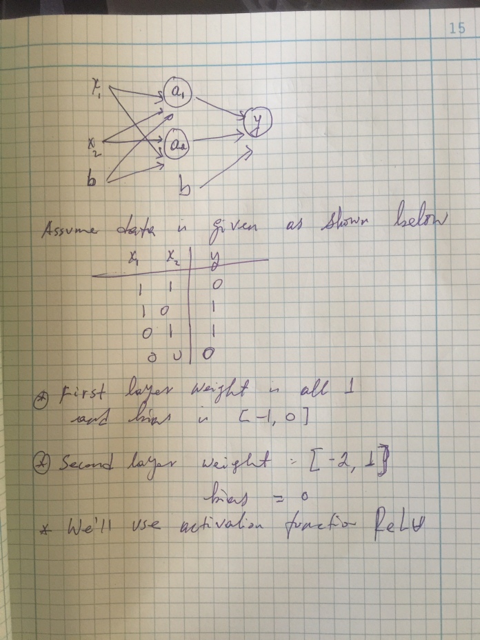Here, we will do forward-propagation for the first input X = [1,1].

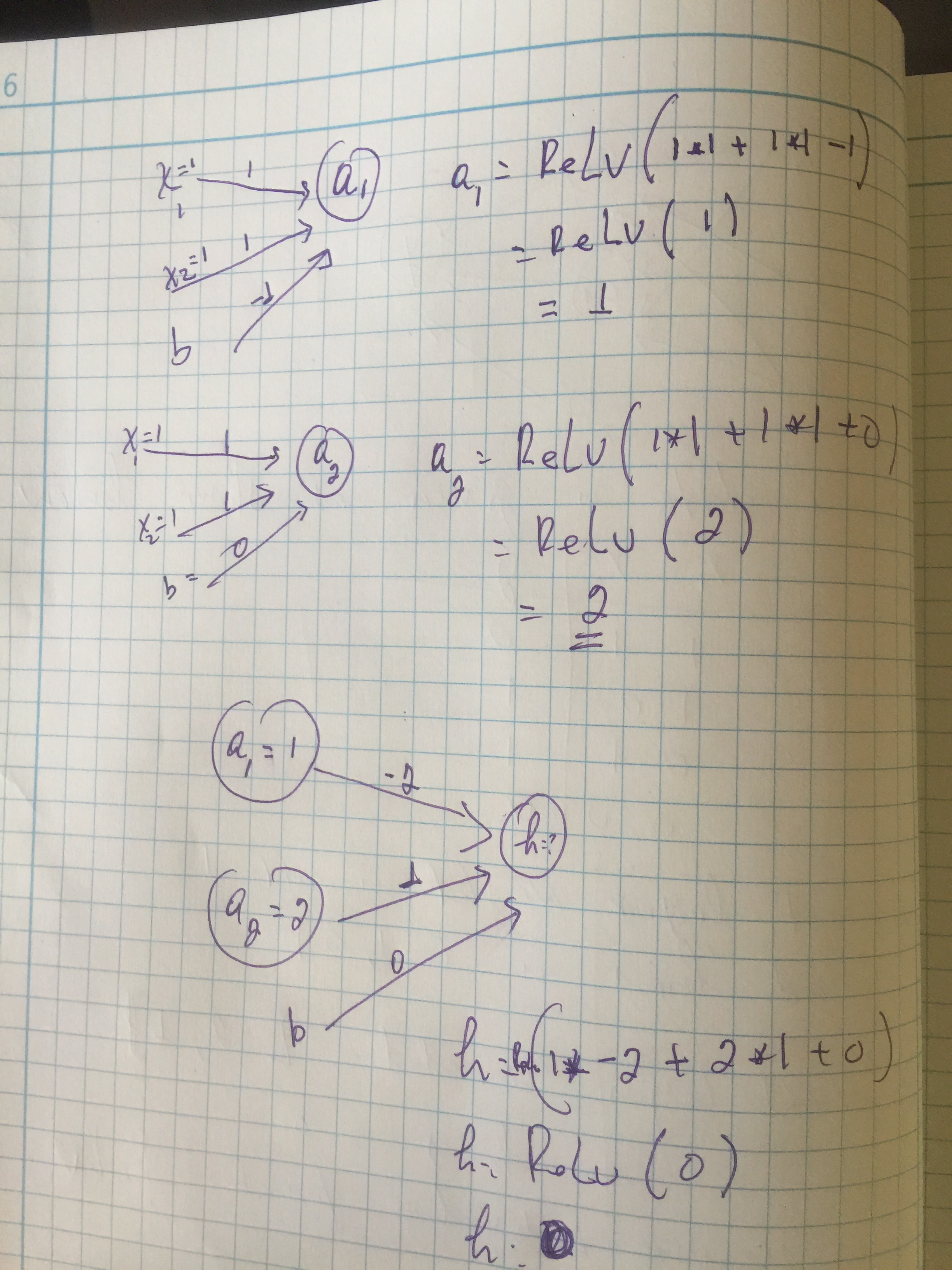
After running the forward propagation, we get a value of 0. Now, the question is what do we do next? Do we penalize the weights or do we keep them as it’s. This is called cost function. We will use the back-propagation to compute the errors induced at each unit.

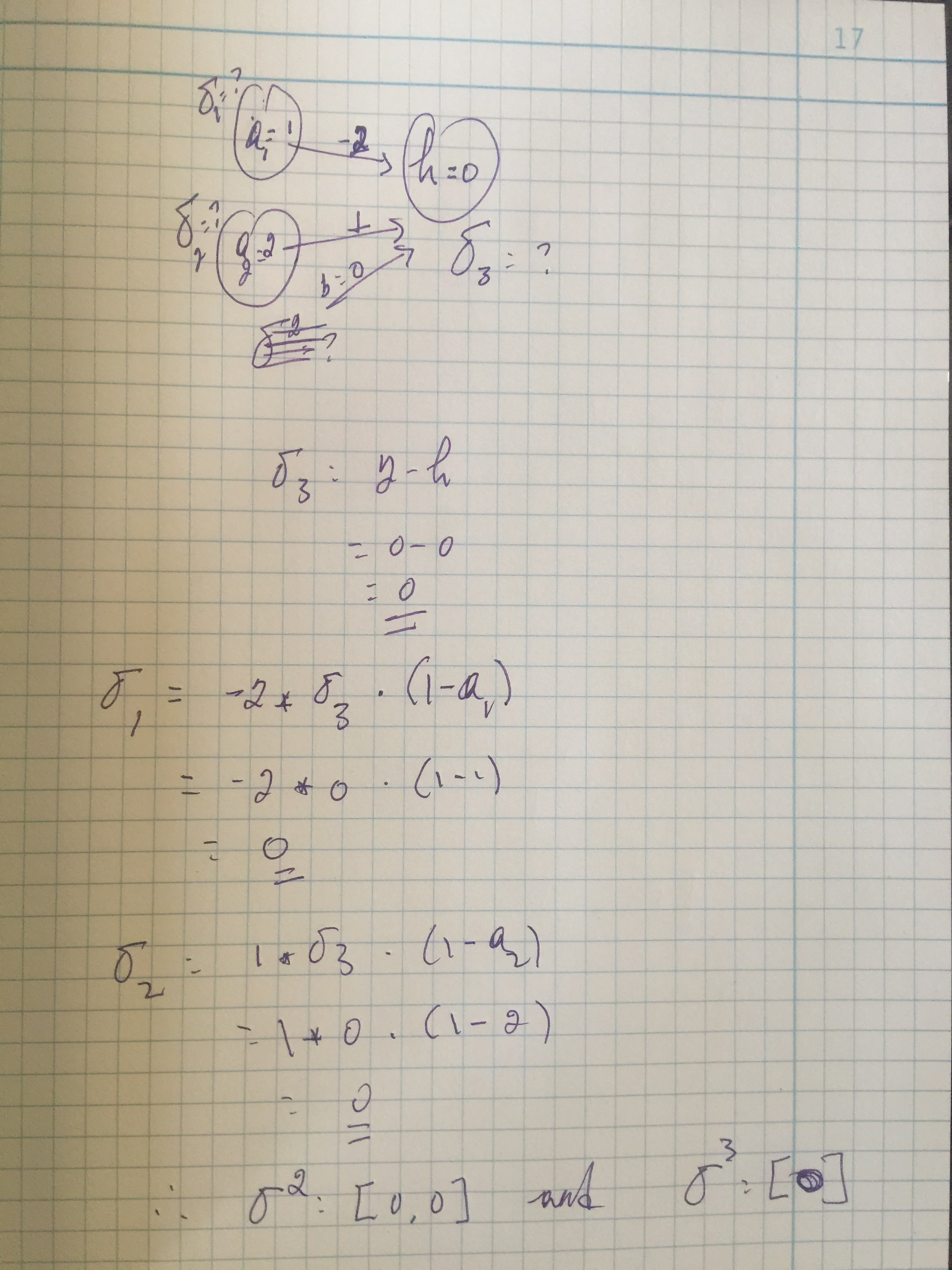
We done. We successfully computed the forward and back propagation algorithm for the input X=[1,1]. This example is taken for the function XOR. Our computation predicted 0 and the output is 0.

For many people forward and back-propagation algorithm may seem very complex but as we have seen in this post, it is not. What makes it complex is the mathematical representations that most people use.

For the data given in this example, the output is an XOR function, which gives 0 if the inputs are equal otherwise 1. In the following plot, we will visualize what the data points look like in the first and hidden layer.

Source: AML4NLP. Red is 0 and blue is 1.

It is interesting to see that the data points in the original space are not linearly separable but they are linearly separable in the hidden space. The take home message for today is that neural networks can handle non-linearity. This is the same notion as in the kernel trick but what is interesting about neural networks is that there is no big dimensions as in kernel trick. Lower dimensions are good for two reasons—more interpretable and better for computation.